Sie suchen eine leistungsstarke Software für anspruchsvolle Aufgaben in Statistik, Grafik, Datenmanagement und automatisierter Berichterstellung?
Dann ist Stata genau das Richtige für Sie! Im Gegensatz zu vielen anderen Programmen bietet Stata zahlreiche Vorteile – überzeugen Sie sich selbst.
Stata Features
NEU in
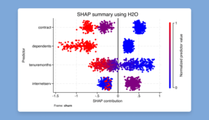
Machine learning via H2O: Ensemble decision trees
What is it?
Machine learning methods are often used to solve research and business problems focused on prediction when the problems require more advanced modeling than linear or generalized linear
models. Ensemble decision tree methods, which combine multiple trees for better predictions, are popular for such tasks. H2O is a scalable machine learning platform that supports data
analysis and machine learning, including ensemble decision tree methods such as random forest and gradient boosting machine (GBM).
The new h2oml suite of Stata commands is a wrapper for H2O that provides end-to-end support for H2O machine learning analysis using ensemble decision tree methods. After using
the h2o commands to initiate or connect to an existing H2O cluster, you can use the h2oml commands to perform GBM and random forest for regression and classification problems. The
h2oml suite offers tools for hyperparameter tuning, validation, cross-validation, evaluating
model performance, obtaining predictions, and explaining these predictions. For example,
Initiate H2O from within Stata
. h20 init
Import data from Stata into H2O
. _h20frame put, into(dataframe) current
Perform gradient boosting binary classification, and tune the number of trees andhyperparameters
. h2oml gbbinclass response predictors, ntrees(20(10)200) lrate(0.1(0.1)1)
Assess variable importance
. h2omlgraph varimp
Make predictions
. _h2oframe change newdata
. h20mlpredict outcome_pred
And there’s much more.
What makes it unique and exciting?
The h2oml suite offers ensemble decision tree methods in an easily accessible way by using familiar Stata syntax or the point-and-click-interface.
With prediction explainability tools such as Shapley additive explanations values, partial dependence plots, and variable importance rankings, GBM and random forest provide powerful
predictions while maintaining explainability—no tradeoffs needed.
Who will use it?
All disciplines; anyone interested in machine learning for classification and regression.
Learn more at stata.com/stata19/h2oml-trees.
For help with setup, also see stata.com/h2o/h2o19/h2o_intro.html.
Conditional average treatment effects (CATE)
What is it?
Treatment effects estimate the causal effect of a treatment on an outcome. This effect may be constant or it may vary across different subpopulations. Researchers are often interested in
whether and how treatment effects differ.
- A labor economist may want to know the effect of a job training program on earnings only for those who participate in the program.
- An online shopping company may want to know the effect of a price discount on purchasing behavior for customers with different demographic characteristics, such as
age and income. - A medical team may want to measure the effect of smoking on stress levels for individuals in different age groups.
With the new cate command, you can go beyond estimating an overall treatment effect to estimating individualized or group-specific ones that address these types of research
questions.
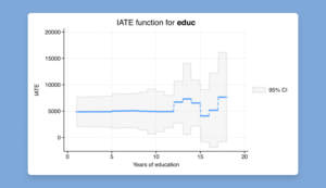
The cate command can estimate three types of CATEs: individualized average treatment effects, group average treatment effects, and sorted group average treatment effects. Beyond
estimation, the cate suite provides features to predict, visualize, and make inferences about the CATEs.
What makes it unique and exciting?
The cate command is powerful, flexible, and treatment models by offering lasso, generalized forest), and parametric models. It provides augmented inverse probability weighting uses cross-fitting to avoid overfitting.
Who will use it?
All disciplines. Anyone interested in causal inference.
Learn more at stata.com/stata19/cate.
High-dimensional fixed effects (HDFE)
What is it?
You can now absorb not just one, but multiple high-dimensional categorical variables in your linear regression, with or without fixed effects, and in linear models accounting for endogeneity
using two-stage least squares. This is useful when you want your model to be adjusted for these variables but estimating their effect is not of interest and is computationally expensive.
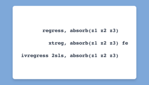
The areg, xtreg, fe, and ivregress 2sls commands now allow the absorb() option to be specified with multiple categorical variables. Previously, areg allowed only one variable in absorb(), while xtreg, fe and ivregress 2sls did not allow the option.
For example, we could fit a regression model that adjusts for three high-dimensional categorical
c1, c2, and c3 predictors by typing
. areg y x, absorb(c1 c2 c3)
If we wanted to absorb these variables in a fixed-effects model, we can do that, too:
. xtset panelvar
. xtreg y x, fe absorb(c1 c2 c3)
And in an instrumental-variables regression model, we can type
. ivregress 2sls y1 x1 (y2 x2), absorb(c1 c2 c3)
What makes it unique and exciting?
Absorbing high-dimensional categorical variables, rather than including indicators for them in your model, results in remarkable speed gains.
Who will use it?
All disciplines. Almost everyone uses linear regression at some point. Economists and political scientists who work with panel data will be especially excited about this new feature.
Learn more at stata.com/stata19/hdfe.
Bayesian variable selection for linear regression
What is it?
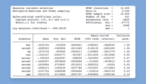
The new bayesselect command provides a flexible Bayesian approach to identify the subset of predictors that are most relevant to your outcome. It accounts for model uncertainty when
estimating model parameters and performs Bayesian inference for regression coefficients. It
uses a familiar syntax,
. bayesselect y x1-x100
As with other Bayesian regression procedures in Stata, posterior means, posterior standard deviations, Monte Carlo standard errors, and credible intervals of each predictor are reported
for easy interpretation. Additionally, either inclusion coefficients or inclusion probabilities, depending on the selected prior, are included to indicate the importance of each predictor to model the outcome.
bayesselect is fully integrated in Stata’s Bayesian suite and works seamlessly with all Bayesian
postestimation routines, including prediction,
. bayesselect pmean, mean
What makes it unique and exciting?
This variable-selection approach offers intuitive interpretation and stable inference.
Who will use it?
Social scientists with large datasets.
Learn more at stata.com/stata19/bayesselect-regress.
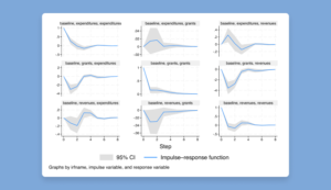
Instrumental-variables local-projection IRFs
What is it?
With the new ivlpirf command, you can account for endogeneity when using local projections to estimate dynamic causal effects.
Local projections are used to estimate the effect of shocks on outcome variables. When the shock of interest is on an impulse variable that may be endogenous, ivlpirf can be used to
estimate the IRFs, and the impulse variable may be instrumented using one or more exogenous instruments.
For example, let’s say we are interested in estimating structural IRFs for the effects of an increase in x on y, using iv as an instrument for the endogenous impulse x:
. ivlpirf y, endogenous(x = iv)
We can then use the irf suite of commands to graph these IRFs:
. irf set ivlp.irf, replace
. irf create ivlp
. irf graph csirf
What makes it unique and exciting?
Estimate dynamic causal effects that account for endogeneity.
Who will use it?
Anyone working with time-series data, including researchers in economics, political science, finance, and public policy.
Learn more at stata.com/stata19/ivlpirf.
Meta-analysis for correlations
What is it?
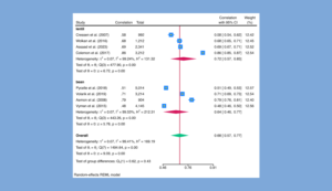
The meta suite now supports meta-analysis of correlation coefficients, allowing investigation of the strength and direction of relationships between variables across multiple studies. For instance, you may have studies reporting the correlation between education and income levels or between physical activity and improvements in mental health and wish to perform meta- analysis.
Say variables corr and ntotal represent the correlation and the total number of subjects in each study, respectively. We can use these variables to declare our data using the meta esize
command.
. meta esize corr ntotal, correlation studylabel(studylbl)
Because the variance of the untransformed correlation depends on the correlation itself, we may prefer to use the Fisher’s z-transformed correlation, a variance-stabilizing transformation
particularly preferable when correlations are close to -1 or 1.
. meta esize corr ntotal, fisherz studylabel(studylbl)
All standard meta-analysis features, such as forest plots and subgroup analysis, are supported.
. meta forestplot, correlation
What makes it unique and exciting?
Correlation studies are a cornerstone in many fields of research. Adding this feature makes meta esize one of the most flexible tools for meta-analysis available.
Who will use it?
All disciplines. Researchers in any discipline may wish to combine results of previous studies to
estimate an overall effect.
Learn more at stata.com/stata19/meta-corr.

Correlated random-effects (CRE) model
What is it?
Easily fit CRE models to panel data with the new cre option of the xtreg command.
Consider the following commands to fit a CRE model with time-varying regressor x and time- invariant regressor z:
. xtset panelvar
. xtreg y x z, cre vce(cluster panelvar)
A random-effects model may yield inconsistent estimates if there is correlation between the covariates and the unobserved panel-level effects. A fixed-effects model wouldn’t allow
estimation of the coefficient on time-invariant regressor z. CRE models offer the best of both worlds.
What makes it unique and exciting?
Estimate coefficients for time-invariant regressors while getting the same coefficients for time-varying regressors as those of xtreg, fe.
Who will use it?
Social scientists and health researchers who work with panel data.
Learn more at stata.com/stata19/cre.
Panel-data vector autoregressive (VAR) model
What is it?
Fit vector autoregressive (VAR) models to panel data! Compute impulse–response functions, perform Granger causality tests and stability tests, include additional covariates, and much
more. The new xtvar command has similar syntax and postestimation procedures as var, but it is appropriate for panel data rather than time-series data.
For example, we could fit a VAR model to a panel dataset with three outcomes of interest by typing
. xtset panelvar
. xtvar y1 y2 y3, lags(2)
Then, we can perform a Granger causality test,
. vargranger
or graph impulse–response functions.
. irf create baseline, set(irfs)
. irf graph irf
What makes it unique and exciting?
Panel-data VAR models have been available through community-contributed commands but have remained a highly requested feature from our users.
Who will use it?
All disciplines. Social scientists who work with panel data will be especially excited about this new feature.
Learn more at stata.com/stata19/panel-var.
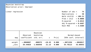
Bayesian bootstrap and replicate weights
What is it?
You can use the new bayesboot prefix to perform Bayesian bootstrap of statistics produced by official and community-contributed commands.
To compute a Bayesian bootstrap estimate of the mean of x, which is returned by summarize
as r(mean), we type
. bayesboot r(mean): summarize x
You can also use the new rwgen command and new options for the bootstrap prefix to implement specialized bootstrap schemes. rwgen generates standard replication and Bayesian
bootstrap weights. bootstrap has new fweights() and iweights() options for performing bootstrap replications using the custom weights. fweights() allows users to specify frequency
weight variables for resampling, and iweights() lets users provide importance weight variables. These options extend bootstrap’s flexibility by allowing user-supplied weights instead of
internal resampling, making it easier to implement specialized bootstrap schemes and enhance reproducibility. bayesboot is a wrapper for rwgen and bootstrap that generates importance
weights using Dirichlet distribution and applies these weights when bootstrapping.
What makes it unique and exciting?
Bayesian bootstrap can be used to obtain more precise parameter estimates in small samples and incorporate prior information when sampling observations.
Who will use it?
All disciplines, especially researchers in statistics, biostatistics, and health fields.
Learn more at stata.com/stata19/bayesboot.
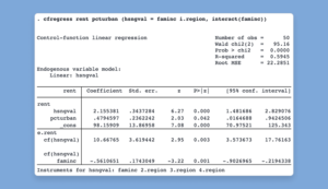
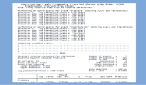
Control-function linear and probit models
What is it?
Fit control-function linear and probit models with the new cfregress and cfprobit commands. Control-function models offer a more flexible approach to traditional instrumental-variables (IV)
methods by including the endogenous variable itself and its first-stage residual in the main regression; the residual term is called a control function.
For example, we could reproduce the estimates of a 2SLS IV regression,
. cfregress y1 x (y2 = z1 z2)
but we could also use a binary endogenous variable and include the interaction of the control
function with z1,
. cfregress y1 x (y2bin = z1 z2, probit interact(z1))
Afterward, we could test for endogeneity by jointly testing the control function and the interaction.
. estat endogenous
What makes it unique and exciting?
First-stage models can be linear, probit, fractional probit, or Poisson, and their control functions can be interacted with other variables or with each other. Robust, cluster–robust, and
heteroskedasticity- and autocorrelation-consistent VCEs are allowed.
Who will use it?
Researchers in the social sciences, particularly economics, public policy, political science, public health, and management.
Learn more at stata.com/stata19/control-functions.
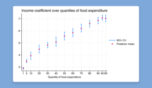
Bayesian quantile regression via asymmetric Laplace likelihood
What is it?
The qreg command for quantile regression is now compatible with the bayes prefix. In the Bayesian framework, we combine the asymmetric Laplace likelihood function with priors to
provide full posterior distributions for quantile regression coefficients.
. bayes: qreg y x1 x2
Consequently, the asymmetric Laplace distribution is also a new likelihood function available in bayesmh.
. bayesmh y x1 x2, likelihood(asymlaplaceq({scale},0.5))
prior({y:}, normal(0,10000)) block({y:})
prior({scale}, igamma(0.01,0.01)) block({scale})
You can also use the asymmetric Laplace likelihood in bayesmh for random-effects quantile regression, simultaneous quantile regression, or to model nonnormal outcomes with
pronounced skewness and kurtosis.
All implementations support standard Bayesian features, such as MCMC diagnostics, hypothesis testing, prediction.
. bayesgraph diagnostics
What makes it unique and exciting?
In classical quantile regression, standard errors are computed using bootstrap or kernel-based methods. In the Bayesian framework, the posterior standard deviations are estimated based on
the model and may be more efficient.
Who will use it?
All disciplines. Researchers in any discipline may be interested in Bayesian analysis.
Learn more at stata.com/stata19/bayes-qreg.
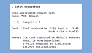
Inference robust to weak instruments
What is it?
To estimate a linear regression of y1 on x1 and endogenous regressor y2 that is instrumented by z1 via 2SLS, we would type
. ivregress 2sls y1 x1 (y2 = z1)
When the instrument, z1, is only weakly correlated with the endogenous regressor, y2, inference can become unreliable even in relatively large samples. The new estat weakrobust
postestimation command after ivregress performs Anderson–Rubin or conditional likelihood- ratio (CLR) tests on the endogenous regressors. These tests are robust to the instrument being
weak.
. estat weakrobust
This postestimation command supports all ivregresss estimators: 2sls, liml, and gmm.
What makes it unique and exciting?
The tests and confidence intervals reported by estat weakrobust not only are robust to weak instruments but also account for the robust, cluster–robust, or heteroskedasticity- and autocorrelation consistent variance–covariance estimator used in ivregress.
Who will use it?
Researchers in the social sciences, particularly economics, public policy, political science, public health, and management.
Learn more at stata.com/stata19/weak-instruments.
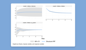
SVAR models via instrumental variables
What is it?
The new ivsvar command estimates the parameters of SVAR models by using instrumental variables.
. ivsvar gmm y1 y2 (shock = z1 z2)
These estimated parameters can be used to trace out dynamic causal effects known as structural impulse–response functions (IRFs) using the familiar irf suite of commands.
. irf set ivsvar.irf
. irf create model1
. irf graph sirf, impulse(shock)
For multiple instruments, use the minimum distance estimator with ivsvar mdist, and specify how the instruments are related to the target shocks.
What makes it unique and exciting?
By relying on instruments, we don’t need to place constraints on the effects of shocks on endogenous variables as in a traditional SVAR model.
Who will use it?
Anyone working with time-series data, including researchers in economics, political science, finance, and public policy.
Learn more at stata.com/stata19/ivsvar.
Mundlak specification test
What is it?
Use the new estat mundlak postestimation command after xtreg to choose between random- effects (RE) and fixed-effects (FE) or correlated random-effects (CRE) models. Unlike a
Hausman test, we do not need to fit both the RE and FE models to perform a Mundlak test—we just need one! Again, consider the following model with time-varying regressor x and time- invariant regressor z:
. xtreg y x z, vce(cluster clustvar)
. estat mundlak
The estat mundlak command ests the null hypothesis that x is uncorrelated with unobserved panel-level effects. Rejecting the hypothesis suggests that fitting an FE or CRE model that accounts for time-invariant unobserved heterogeneity is more sensible than an RE model.
What makes it unique and exciting?
Unlike the Hausman test for FE versus RE, the Mundlak test provides valid inference with cluster–robust, bootstrap, and jackknife standard errors.
Who will use it?
Social scientists and health researchers who work with panel data, particularly economists and political scientists.
Learn more at stata.com/stata19/mundlak.
Latent class model-comparison statistics
What is it?
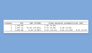
When you perform latent class analysis or finite mixture modeling, it is fundamental to determine the number of latent classes that best fits your data. With the new lcstats
command, you can use statistics such as entropy and a variety of information criteria, as well as the Lo–Mendell–Rubin (LMR) adjusted likelihood-ratio test and Vuong–Lo–Mendell–Rubin (VLMR) likelihood-ratio test, to help you determine the appropriate number of classes. For example, you might fit one-class, two-class, and three-class models and store their results by typing
. gsem (y1 y2 y3 y4 <- ), logit lclass(C 1)
. estimates store oneclass
. gsem (y1 y2 y3 y4 <- ), logit lclass(C 2)
. estimates store twoclass
. gsem (y1 y2 y3 y4 <- ), logit lclass(C 3)
. estimates store threeclass
Then you can obtain model-comparison statistics and tests by typing
. lcstats
The lcstats command offers options for specifying which statistics and test to report and to customize the look of the table.
What makes it unique and exciting?
This has been the most requested addition to our latent class analysis features since they were first released.
The tables produced by lcstats are automatically placed in a collection, which means they are very easy to further customize and to export to a variety of file types by using the collect
commands.
Who will use it?
Researchers in behavioral sciences, health, and business often use latent class analysis, while social scientists and statisticians use finite mixture modeling. This feature will be useful to
anyone performing these types of analysis.
Learn more at stata.com/stata19/lcstats.
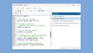
Do-file Editor: Autocompletion, templates, and more
What is it?
The Do-file Editor has the following additions:
Autocompletion of variable names, macros, and stored results. If you pause briefly as you type, suggestions of variable names from data in memory, macros, and stored results will appear in addition to the command names and existing words that appeared previously.
Do-file Editor templates. You can now save time and ensure consistency when you create new documents in the Do-file Editor by using Stata templates and user-defined templates.
Do-file Editor current word and selection highlighting. The Do-file Editor will now highlight all case-insensitive occurrences of the current word under the cursor and all case-sensitive occurrences of the current selection.
Bracket highlighting. The Do-file Editor will now highlight the brackets enclosing the current cursor position as you move through the document.
Code folding enhancements. You can now quickly fold all foldable blocks of code in your do- file by using the Fold all menu item. You can then selectively unfold your code one fold point at a time to show the more important parts of your do-file, or you can use the Do-file Editor’s Unfold all menu item to unfold every fold point. You can also select lines of code and transform them into a foldable block of code by using the Fold selection menu item. This can tidy up your code and increase the code’s readability. In addition, the code-folding feature has been changed to be less visually distracting by using arrow markers in the code-folding ribbon to indicate whether a code fold is expanded or collapsed and to hide expanded code-fold markers unless the user hovers the mouse over the code-folding ribbon.
Do-file Editor temporary and permanent bookmarks. The Do-file Editor now supports temporary bookmarks in addition to permanent bookmarks. The existing permanent
bookmarks are saved as part of the do-file. You can use the new temporary bookmarks to immediately navigate your do-file but without making any changes to its content.
Show whitespace and tabs. The Do-file Editor can now show whitespace characters only within a selection instead of always showing them or not showing them at all.
Navigator panel. The Navigation control from previous releases of Stata has been replaced by the Navigator panel. It displays a list of permanent bookmarks and programs that are in a do-
file. You can quickly jump to the position of a program or bookmark by double-clicking on the item in the Navigator panel. You can also delete and indent bookmarks from the Navigator
panel.
What makes it unique and exciting?
The Do-file Editor is a much-used tool for writing a script containing a series of Stata commands or even an ado-file that defines a new command. New features in the Do-file Editor make Stata coding more efficient and make the user’s experience of writing code better.
Who will use it?
All Stata users.
Learn more stata.com/stata19/do-file-editor.
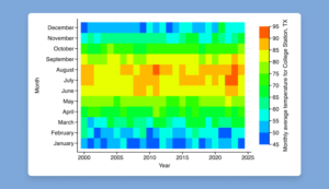
Graphics: Bar graph CIs, heat maps, and more
What is it?
Stata 19 includes many new graphics features.
Heat maps. The new twoway heatmap command creates a heat map, which displays values of a numeric variable, z, across values of y and x as a grid of colored rectangles.
Range and point plot with capped spikes. The new twoway rpcap command plots points and range indicated by spikes with caps. These plots are useful for displaying a value of
interest, such as a mean, and the corresponding confidence interval.
Range and point plot with spikes. The new twoway rpspike command plots points and ranges indicated by spikes. These plots are useful for displaying a value of interest, such as a
mean, and the corresponding confidence interval.
Bar graphs with CIs, improved labeling, and control of bar groupings. graph bar now allows you to graph the mean and corresponding confidence interval. You can also use the new groupyvars option to group bars for the same y variable together. graph bar also has new options to control the ticks and labels on the categorical axis and to add a prefix or suffix to the
bar labels.
Dot charts with CIs, improved labeling, and control of dot groupings. graph dot now allows you to graph the mean and corresponding confidence interval. You can also use the new
groupyvars option to group dots for the same y variable together. graph dot also has new options to control the ticks and labels on the categorical axis.
Box plots with improved labeling and control of box groupings. You can also use the new groupyvars option to group boxes for the same y variable together. graph box also has new
options to control the ticks and labels on the categorical axis.
Colors by variable for more graphs. The colorvar() option is now available with more twoway plots: line, connected, tsline, rline, rconnected, and tsrline. This option allows plots to vary color
of lines, markers, and more based on the values of a specified variable.
What makes it unique and exciting?
These are some of the most requested additions to our features for graphics. In particular, the confidence intervals and new bar-grouping options for bar graphs have been a repeat request. Heat maps are also popular.
Who will use it?
Almost every researcher creates graphs. These new features will appeal to all disciplines.
Learn more at stata.com/stata19/graphics.
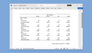
Tables: Easier tabulations, exporting, and more
What is it?
Stata 19 also includes many additions that allow users to more easily create and customize tables.
Titles, notes, and exporting for tables. The table command is a flexible tool for creating tabulations, tables of summary statistics, tables of regression results, and more. It now allows you to add a title with the new title() option, to add a note with the new note() option, to control the appearance of the title and notes with the new titlestyles() and notestyles() options, and to export your table to your preferred document type (Word, LaTeX, Excel, etc.) with the new export() option.
Easier ANOVA tables. You can now more easily create and customize ANOVA tables afte anova and oneway by collecting the new stored matrix r(ANOVA). You can use the new anova
collection style to easily format these results in a standard ANOVA-style layout.
Better labels with collect get. With command collect get’s new option commands(), you can specify the command names that posted the results being consumed. This allows collect get
to search for command-specific result labels. The results in the collection will often have better labels, as they would if the collect prefix were used instead of the collect get command.
Determine layout of a collection. The new collect query layout command allows you to query a collection’s layout specification. Previously, users typed collect layout to display both the layout and the table. Now you no longer need to see the full table each time you want to see the layout.
Control factor variables in headers. With collect style header’s new option fvlevels(), you have more control over how factor variables appear in a table. Specify whether to hide or show
factor-variable levels in row and column headers.
Remove results from a collection. The new collect unget command allows you to remove selected results from a collection. This can make it easier to lay out tables that do not involve these results.
Table-specific notes. The collect notes command has the new fortags() option that allows you to control which table should show the specified note.
Tabulations with measures of association and tests. You can now easily create customized tables with the results of tabulate and svy: tabulate. With the new collect() option, tabulated
statistics are stored in a collection with its own layout and styles, which can be further customized and exported to a variety of file types. This is particularly useful when you wish to include cumulative percentages or measures of association from tabulate and tests from svy: tabulate.
What makes it unique and exciting?
These are some of the most requested additions to our features for generating tables.
Who will use it?
Almost every researcher needs to present results clearly through tables. These new features will appeal to all disciplines.
Learn more at stata.com/stata19/tables.
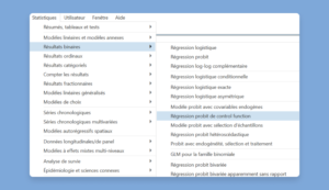
Stata in French
What is it?
Stata’s menus, dialogs, and the like can now be displayed in French. If your computer language is set to French (fr), Stata will automatically use its French setting. To
change languages manually using Windows or Unix, select Edit > Preferences > User- interface language…. If you are using MacOS, select Stata 19 > Preferences > User-interface language…. You can also change the language from the command line by using the set locale_ui command.
Who will use it?
Any researchers who speak French.
Learn more at stata.com/stata19/french.
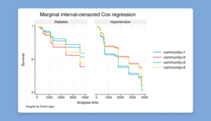
Interval-censored multiple-event Cox model
Einsatzbereiche
Forscher verschiedenster Disziplinen setzen seit mehr als 40 Jahren auf Stata Software. Und das mit Erfolg, denn Stata bietet ihnen alles, was sie im Bereich Datenmanagement, Visualisierung, Statistik und automatisierte Berichterstellung benötigen.
Womit beschäftigen Sie sich? Finden Sie heraus, was Stata für Sie tun kann:


Warum Stata?
Hochwertige Grafiken
Mit Stata erstellen Sie qualitativ hochwertige Diagramme für Publikationen und interne Dokumente. Sie können jederzeit zwischen vordefinierten oder selbst eingestellten Diagrammtypen wählen. Mit dem integrierten Grafik-Editor können Sie die Diagramme per Mausklick individualisieren und Titel, Notizen, Linien, Pfeile und Text hinzufügen. Mit selbstgeschriebenen Scripten lassen sich tausende Grafiken erzeugen (reproduzierbar) und exportieren – als EPS oder TIF für Publikationen, als PNG für das Internet oder auch PDF.
Schnell, genau und einfach zu benutzen
Dank seiner benutzerfreundlichen Oberfläche und der intuitiven Befehlssyntax ist Stata besonders einfach zu bedienen. Stata liefert genaue statistische Ergebnisse in Hochgeschwindigkeit. Die Ergebnisse können Sie mit minimalem Aufwand dokumentieren und für Veröffentlichungen reproduzieren. Stata’s Online-Hilfe und weitere Online-Ressourcen unterstützen bei der Auswertung komplexer Fragestellungen.
Umfassendes Datenmanagement
Die Datenmanagement-Befehle in Stata ermöglichen dem Anwender die vollständige Kontrolle aller möglichen Datentypen: Man kann Datensets kombinieren und umordnen, Variablen verwalten und statistische Auswertungen über Gruppen oder Replikate hinweg ausführen. Stata beinhaltet zudem erweiterte leistungsstarke Werkzeuge für die Arbeit mit speziellen Daten wie Survival-, Zeitreihen-, Panel-/Longitudinal-, Multiple-Imputation-, kategoriale und Survery-Daten.
Echte reproduzierbare Forschung
Betriebssystem-übergreifend einsetzbar
Stata läuft unter Windows, Mac und Unix-Betriebssystemen (inkl. Linux). Stata-Lizenzen sind plattform-unabhängig. Stata-Datensätze, Programme und andere Daten können betriebssystem-übergreifend ohne weitere Übersetzung genutzt werden. Datensätze aus anderen Statistikprogrammen, Tabellen und Datenbanken lassen sich schnell und einfach importieren.
Matrix-Programmiersprache: Mata
Sie müssen zwar nicht programmieren, um Stata verwenden zu können, dennoch bietet Stata Ihnen mit Mata eine schnelle und vollständige Matrix-Programmiersprache. Mata ist beides – eine interaktive Umgebung zur Bearbeitung von Matrizen und eine komplette Entwicklungsumgebung zur Erstellung von kompiliertem und optimiertem Programmcode. Mata beinhaltet spezielle Features, um Paneldaten zu verarbeiten und Operationen auf reellen oder kompletten Matrizen durchzuführen. Mata unterstützt eine objektorientierte Programmierung und bietet eine vollständige Integration mit allen Stata relevanten Funktionalitäten und Charakteristika.
Erweiterbar
Stata ist so einfach zu programmieren, dass Entwickler und Nutzer täglich neue Features hinzufügen, um die Anforderungen der Anwender zu erfüllen. Neue Features und offizielle Updates können kostenlos aus dem Internet mit einem einzigen Klick heruntergeladen und installiert werden. Das quartärlich erscheinende Stata Journal informiert Sie über neue Features und aktuelle Anwendungsbeispiele. Über die Statalist, einem unabhängigen Listserver, tauschen Stata-User Informationen und Programme aus.
Ressourcen
Editionen

Stata BE
Basic Edition für mittelgroße Datensätze
Mit Stata BE lassen sich Datendateien mit bis zu 2.048 Variablen auswerten. Die Anzahl der Beobachtungen ist nur durch die RAM-Größe Ihres Rechners begrenzt. Stata BE kann maximal 798 unabhängige Variablen in einem Modell verarbeiten.

Stata SE
Standard Edition für größere Datensätze
Stata SE und Stata BE unterscheiden sich vor allem hinsichtlich der Größe der analysierbaren Datendateien. Mit Stata SE lassen sich Datendateien mit bis zu 32.767 Variablen und maximal 10.998 unabhängige Variablen in einem Modell verarbeiten.

Stata MP
Die schnellste Edition mit der die größten Datensätze analysiert werden können
(Für Quad-Core-, Dual-Core- und Multicore- / Multiprozessor-Computer)
Stata MP ist die schnellste und leistungsstärkste Stata-Version. Stata MP läuft auf Dual-Core-Computern (Intel Core 2 Duo, i3, i5, i7, i9, Xeon, Celeron, AMD X2) rund 40% schneller. Sogar 72% Beschleunigung erreicht Stata MP bei den zeitaufwändigen Estimation-Befehlen. Noch schnellere Analysen erzielt Stata MP auf Multi-Core- und Multiprozessor-Systemen. Stata MP verarbeitet Datendateien mit bis zu 65.532 Variablen und erstellt Modelle mit maximal 120.000 unabhängigen Variablen.
Stata MP
Stata holt das Beste aus Multicore-Systemen heraus.
Keine andere Statistiksoftware kommt dem auch nur nahe.
Stata MP ist die schnellste und umfangreichste Edition von Stata.
Nahezu jeder Computer kann die fortschrittlichen Multiprocessing-Fähigkeiten von Stata/MP nutzen. Stata/MP bietet die umfassendste Multicore-Unterstützung aller Statistik- und Datenverarbeitungspakete.
Geschwindigkeit
Stata MP ist schneller – viel schneller.
Mit Stata/MP können Sie Daten in kürzerer Zeit analysieren – sowohl auf kostengünstigen Multicore-Laptops und Desktop-Computern als auch auf Multiprozessor-Servern. Nutzen Sie nur 2 Kerne, so laufen Ihre Analysen in der Hälfte bis zwei Dritteln der Zeit im Vergleich zu Stata SE. Nutzen Sie 4 Kerne, so verkürzt sich die Zeit auf ein Viertel bis die Hälfte. Nutzen Sie noch mehr Kerne für noch schnellere Analysen. Stata/MP unterstützt bis zu 64 Kerne/Prozessoren.
Geschwindigkeit ist oft dann am entscheidendsten, wenn rechenintensive Schätzverfahren durchgeführt werden. Einige der Schätzverfahren von Stata – darunter die lineare Regression – sind nahezu perfekt parallelisiert; das bedeutet, sie laufen auf 2 Kernen doppelt so schnell, auf 4 Kernen viermal so schnell, auf 8 Kernen achtmal so schnell und so weiter. Manche Schätzbefehle lassen sich stärker parallelisieren als andere. Betrachtet man den Median, so laufen Schätzbefehle auf 2 Kernen 1,7-mal schneller, auf 4 Kernen 2,6-mal schneller und auf 8 Kernen 3,4-mal schneller.
Auch bei der Verwaltung großer Datensätze kann Geschwindigkeit eine wichtige Rolle spielen. Das Hinzufügen neuer Variablen ist zu nahezu 100 % parallelisiert, und das Sortieren ist zu 61 % parallelisiert.
Einige Verfahren sind nicht parallelisiert, und manche sind naturgemäß sequenziell angelegt; dies bedeutet, dass sie in Stata/MP mit derselben Geschwindigkeit ablaufen.
Für eine umfassende Bewertung der Leistung von Stata/MP – einschließlich detaillierter Statistiken für jeden einzelnen Befehl – lesen Sie bitte den „Stata MP Performance Report“.
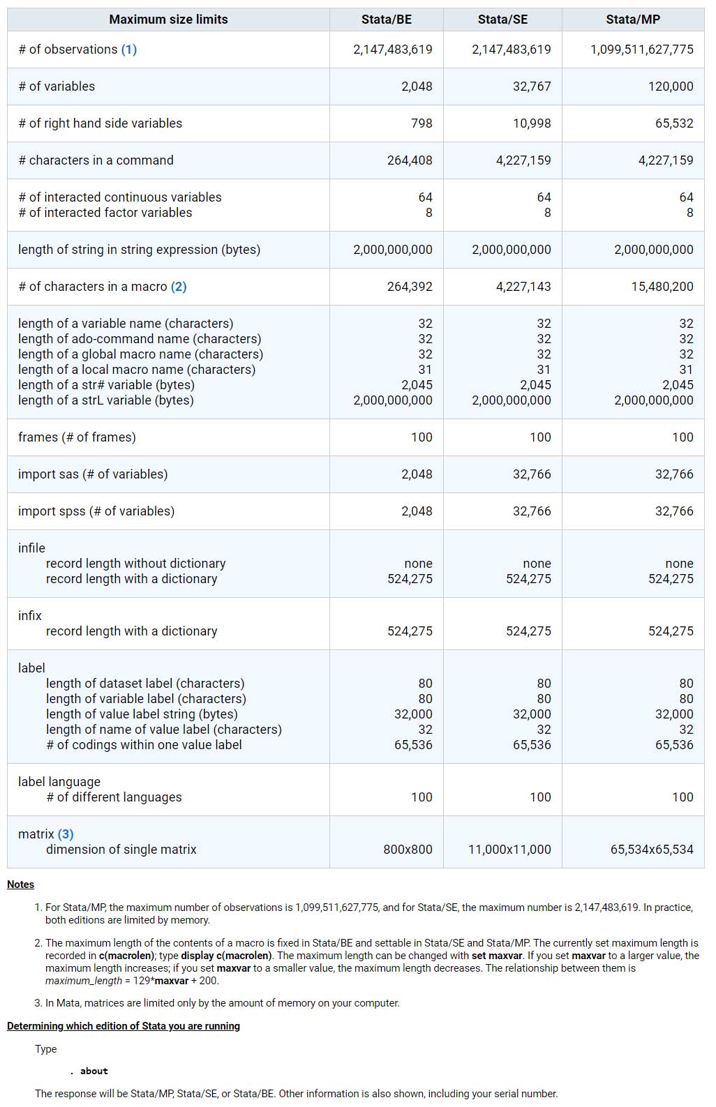
Größe
Da Geschwindigkeit dann am wichtigsten ist, wenn Ihre Probleme groß sind, unterstützt Stata MP noch größere Datensätze als Stata SE.
Stata SE kann bis zu 2 Milliarden Beobachtungen analysieren. Stata MP kann auf den derzeit leistungsstärksten Computern 10 bis 20 Milliarden Beobachtungen analysieren und ist darauf vorbereitet, bis zu 1 Billion Beobachtungen zu verarbeiten, sobald die Computerhardware entsprechend nachgezogen hat. Zudem erlaubt Stata MP 120.000 Variablen – im Vergleich zu den 32.767 Variablen, die von Stata SE unterstützt werden.
| Max. no. of variables | Max. no. of independent variables | Max. no. of observations | |
|---|---|---|---|
| Stata/MP | 120,000 | 65,532 | 20 billion* |
| Stata/SE | 32,767 | 10,998 | 2.14 billion |
| Stata/BE | 2,048 | 798 | 2.14 billion |
*The maximum number of observations is limited by the amount of available RAM on your system.
Kompatibilität
Stata MP ist zu 100 % mit anderen Editionen von Stata kompatibel.
Analysen müssen in keiner Weise neu formuliert oder modifiziert werden, um die Geschwindigkeitsvorteile von Stata/ P zu nutzen.
Platforms
Stata/MP ist für die folgenden Betriebssysteme verfügbar:
✓ Windows (64-bit) ✓ macOS (Apple Silicon and 64-bit) ✓ Linux (64-bit)
Das heißt konkret: für alle von Stata unterstützten Plattformen.
Um Stata/MP auszuführen, können Sie entweder einen Desktop-Computer mit einem Dual-Core- oder Quad-Core-Prozessor verwenden oder einen Server mit mehreren Prozessoren. Ob ein Computer über separate Prozessoren oder über einen einzelnen Prozessor mit mehreren Kernen verfügt, macht dabei keinen Unterschied. Eine höhere Anzahl an Prozessoren oder Kernen sorgt dafür, dass Stata/MP schneller läuft.
Weitere Empfehlungen zur Hardware finden Sie in unserem Abschnitt zur Hardware für Stata MP.

Systemanforderung
Stata for Windows
- Windows 11*
- Windows 10*
- Windows Server 2022, 2019, 2016, 2012R2*
* 64-bit for x86-64 made by Intel® and AMD
Stata for Mac
- Mac with Intel processor or Apple Silicon
- Stata for Linux“ to „macOS 11 (Big Sur) through macOS 26 (Tahoe) for Macs with Apple Silicon and macOS 10.13 (High Sierra) through macOS 26 (Tahoe) for Macs with Intel processors“
Stata for Linux
- 64-bit (x86-64)
- Minimum requirements include the GNU C library (glibc) 2.28 or better and libcurl4
- For xstata, you need to have GTK 2.24 installed
Hardware-requirements
- Minimum of 1 GB of RAM für IC, 2 GB RAM für SE, 4 GB RAM für MP
- Minimum of 4 GB of disk space
- Stata for Unix requires a video card that can display thousands of colors or more (16-bit or 24-bit color)
Hardware-Empfehlungen für Dual-core-, Multi-core oder Multiprozessor-Computer

DPC Software GmbH
Offizieller Stata Distributor
für Deutschland, Niederlande, Österreich, Tschechien und Ungarn
Jetzt Stata bequem im Onlineshop kaufen.
Egal ob Student, Prof+Plan, Educational oder Business –
In unserem Onlineshop finden Sie die passende Lizenz für Ihren Bedarf!
Bei Fragen hilft Ihnen unser Stata-Sales-Team gerne weiter: order@dpc-software.de
Stata Testversion
Überzeugen Sie sich selbst und fordern Sie
Ihre eine Stata Testversion von kostenlos für 30 Tage an.
Ihre Anfrage
Erhalten Sie ein unverbindliches Angebot.
Zugeschnitten auf Ihren Bedarf und Ihr Unternehmen.
Onlineshop
Kaufen Sie Stata für akademische oder nichtakademische Zwecke. Wir bieten auch spezielle Rabatte für Studenten über unseren Online-Shop an